DuckDB Architecture — Why It's So Fast

Introduction

Why is DuckDB so fast? Despite being usable with just pip install, how can it process large-scale data aggregations at high speed? This article explains its internal architecture.

DuckDB’s design is based on the 2020 paper Data Management for Data Science — Towards Embedded Analytics (CIDR 2020). The core of its speed comes down to three key elements:

1. Columnar Storage — Read only the columns you need
2. Vectorized Execution — Batch processing in units of 2048 rows
3. Query Optimizer — Eliminate unnecessary operations in advance

What Is Columnar Storage?

Row-Oriented vs. Column-Oriented

Traditional databases (MySQL, PostgreSQL, etc.) use row-oriented storage, where each row’s data is stored contiguously on disk.

Row Store
┌──────────────────────────────────────┐
│ id=1, name="Alice",  score=95.5, ... │  ← Row 1
│ id=2, name="Bob",    score=87.0, ... │  ← Row 2
│ id=3, name="Charlie",score=92.3, ... │  ← Row 3
└──────────────────────────────────────┘

DuckDB uses columnar storage, where data from the same column is stored contiguously.

Column Store
┌────────────────────────┐
│ id:    1,  2,  3, ...  │  ← id column
│ name:  Alice, Bob, ... │  ← name column
│ score: 95.5, 87.0, ... │  ← score column
└────────────────────────┘

Why Analytical Queries Become Faster

Consider an aggregation query like SELECT AVG(score) FROM users.

• Row-oriented: All rows must be read to extract only score. id and name are read unnecessarily
• Column-oriented: Only the score column is read sequentially. I/O is minimized

Furthermore, since data of the same type is stored contiguously, compression efficiency improves dramatically.

Vectorized Execution

Row-at-a-Time vs. Batch Processing

Traditional databases primarily used “row-at-a-time” processing (the Volcano Model).

Traditional Model (Volcano Model)
  Query Execution Engine
    ↓ Request 1 row
  Filter Node
    ↓ Request 1 row
  Scan Node
    → Returns 1 row at a time

DuckDB uses “vectorized execution,” processing 2048 rows at once.

Vectorized Execution
  Query Execution Engine
    ↓ Request 2048 rows at once
  Filter Node (evaluate 2048 rows in bulk with SIMD)
    ↓ Resulting 2048 rows
  Scan Node
    → Returns 2048 rows in bulk

The advantages of this approach are as follows:

SIMD (Single Instruction, Multiple Data)

Modern CPUs can process multiple data elements simultaneously with a single instruction (SIMD). Vectorized execution leverages this to the fullest.

SIMD Operation Example (128-bit SIMD adding 4 int32 values simultaneously)
[1, 2, 3, 4]
[5, 6, 7, 8]
     ↓ SIMD addition (1 instruction)
[6, 8, 10, 12]

Query Optimizer

DuckDB optimizes queries before execution, removing unnecessary operations.

Predicate Pushdown

Filter conditions are applied as early as possible.

SELECT name FROM users WHERE score > 90;

Before optimization:

Full table scan → JOIN/aggregation → Filter (score > 90) → Retrieve name

After optimization:

Filter (score > 90) during scan → Process only matching rows → Retrieve name

The amount of data read is significantly reduced.

Projection Pushdown

Columns not used in the query are never read in the first place.

SELECT name, score FROM users;  -- id is not needed

The id column is not read from disk. This is especially effective when combined with columnar storage.

Parallel Query Execution

DuckDB automatically utilizes multiple cores. By default, it uses as many threads as logical cores to execute queries in parallel.

import duckdb

# Check the number of threads
con = duckdb.connect()
print(con.execute("SELECT current_setting('threads')").fetchone())
# → ('4',)

Scans and aggregations on large tables are automatically partitioned and processed in parallel across cores.

Memory Management and Out-of-Core Processing

DuckDB can process large-scale data that doesn’t fit in memory.

• Buffer Pool: Caches frequently accessed data in memory
• Out-of-Core Processing: Spills to disk and continues execution when memory is insufficient
• Memory Limit Configuration: Can be explicitly limited with SET memory_limit='4GB'

SET memory_limit = '4GB';
SET threads = 2;

TPC-H Benchmark Results

TPC-H is an industry-standard benchmark for OLAP performance. Using DuckDB’s tpch extension, everything from data generation to query execution can be done in one place.

import duckdb, time

con = duckdb.connect()
con.execute('INSTALL tpch; LOAD tpch;')
con.execute('CALL dbgen(sf=1);')  # Specify Scale Factor with sf=N

The Scale Factor (SF) is a multiplier for the amount of data generated. SF=1 generates approximately 6 million rows in the lineitem table.

Benchmark Queries

Execution time was measured with three types of queries.

Q1: Full Table Scan + Aggregation (reads all rows of lineitem and performs group aggregation)

SELECT l_returnflag, l_linestatus,
       COUNT(*) AS count_order, SUM(l_quantity) AS sum_qty
FROM lineitem
WHERE l_shipdate <= DATE '1998-09-02'
GROUP BY l_returnflag, l_linestatus
ORDER BY l_returnflag, l_linestatus;

Q6: Filtered Aggregation (single aggregation after applying filter conditions)

SELECT SUM(l_extendedprice * l_discount) AS revenue
FROM lineitem
WHERE l_shipdate >= DATE '1994-01-01'
  AND l_shipdate < DATE '1995-01-01'
  AND l_discount BETWEEN 0.05 AND 0.07
  AND l_quantity < 24;

Q5: 6-Table JOIN + Aggregation (the most complex query)

SELECT n_name, SUM(l_extendedprice * (1 - l_discount)) AS revenue
FROM customer, orders, lineitem, supplier, nation, region
WHERE c_custkey = o_custkey
  AND l_orderkey = o_orderkey
  AND l_suppkey = s_suppkey
  AND c_nationkey = s_nationkey
  AND s_nationkey = n_nationkey
  AND n_regionkey = r_regionkey
  AND r_name = 'ASIA'
  AND o_orderdate >= DATE '1994-01-01'
  AND o_orderdate < DATE '1995-01-01'
GROUP BY n_name ORDER BY revenue DESC;

Measured Results (SF=0.1 to SF=20)

Average values from three measurements at each SF are recorded below.

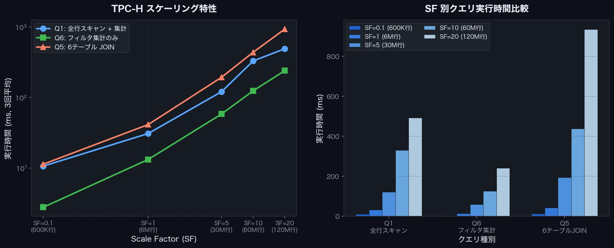Execution time comparison of Q1/Q6/Q5 for TPC-H SF=0.1–20 (DuckDB v1.4.4)

When SF increases by 10x, execution time increases by roughly 10–20x. Q5 (6-table JOIN) is most affected by data volume growth, reaching 934ms at SF=20. Meanwhile, Q6 (simple filtered aggregation) remains relatively contained at 240ms.

Thanks to I/O reduction from columnar storage and SIMD vectorization, Q1 aggregation on 120 million rows completes within 500ms.

Relationship with Apache Arrow

DuckDB internally leverages Apache Arrow’s columnar format.

• Zero-Copy Transfer: Data can be transferred to and from Pandas or Polars without copying
• Interoperability: High-speed integration with other tools via the Arrow format
• Memory Efficiency: Directly utilizes Arrow’s efficient memory layout

import duckdb

con = duckdb.connect()
# Retrieve as Arrow Table (zero-copy)
arrow_table = con.execute("SELECT * FROM range(1000000) t(i)").fetch_arrow_table()
print(arrow_table.schema)

Summary

DuckDB’s speed comes from the combination of the following technologies:

Aggregating 600K rows takes around 10ms, and even over 100 million rows completes within a few hundred milliseconds. The fact that this performance is available without a server and with a single-line install is what makes DuckDB so compelling.

References

Why DuckDB

Why DuckDB There are many database management systems (DBMS) out there. But there is no one-size-fits-all database system. All take different trade-offs to better adjust to specific use cases. DuckDB is no different. Here, we try to explain what goals DuckDB has and why and how we try to achieve those goals through technical means. To start with, DuckDB is a relational (table-oriented) DBMS that supports the Structured Query Language (SQL). Key Characteristics of DuckDB Simple SQLite is the world's most widely deployed DBMS. Simplicity in installation, and embedded in-process operation are central to its success. DuckDB adopts these ideas…

duckdb.org

https://duckdb.org/pdf/CIDR2020-raasveldt-muehleisen-duckdb.pdf

duckdb.org

Redirecting…

duckdb.org